Residplot Examples

publiplots.residplot() wraps seaborn.residplot() — the scatter of regression residuals — and extends it with a hue= dimension that seaborn doesn’t natively support. Each hue level gets its own residual computation and a palette-mapped color; a categorical hue legend is auto-rendered via the publiplots legend reactor.

Use residplot to diagnose fit quality: curvature in the residual cloud (or a noticeable LOWESS bow) suggests the current regression order is too low; obvious heteroscedasticity hints that variance isn’t constant across the predictor.

import publiplots as pp
from publiplots.plot.residplot import residplot
import numpy as np
import pandas as pd

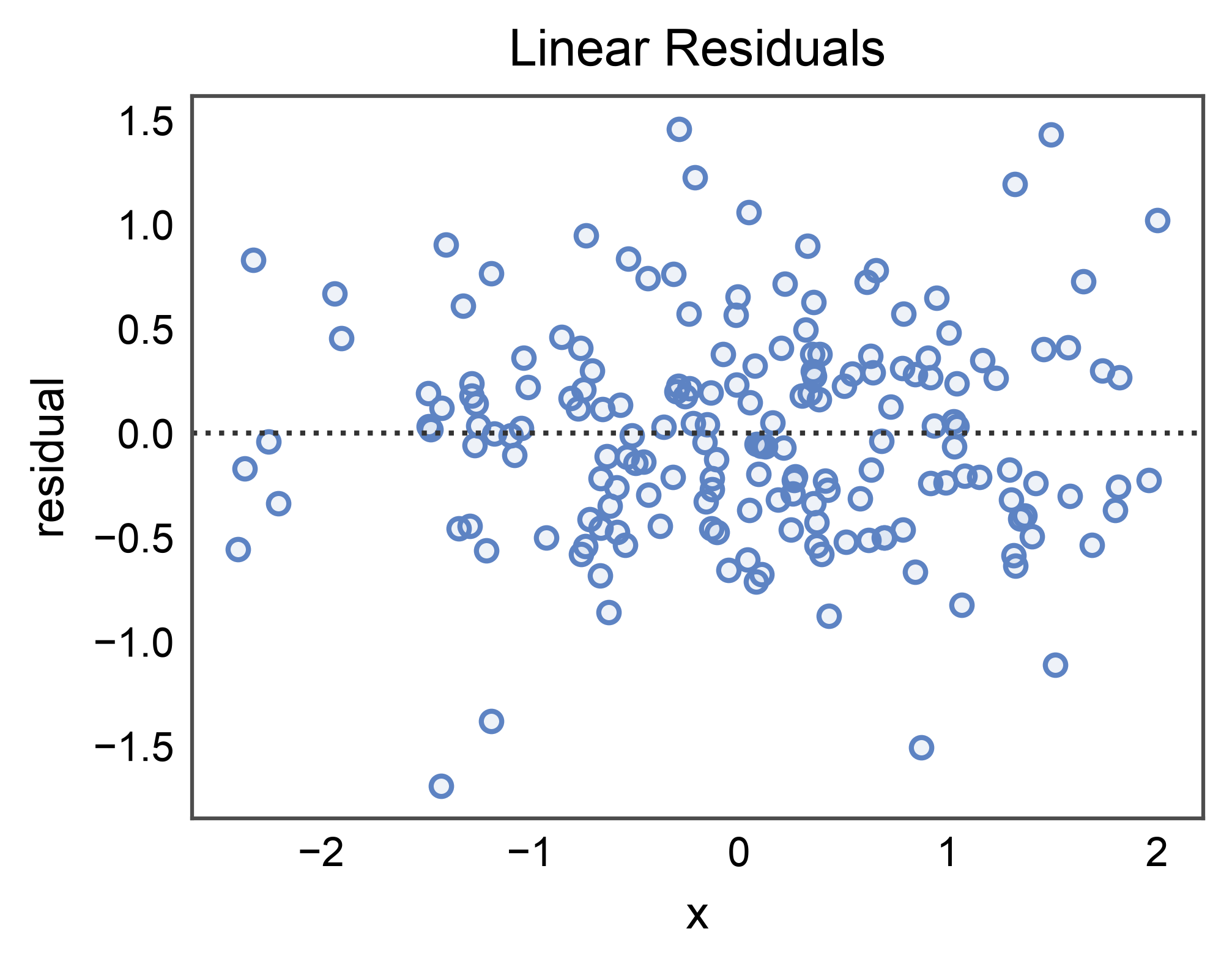
Basic Residuals (Linear Fit)

The simplest case: residuals of a linear regression of y on x. The dotted horizontal is the zero reference line (a well-fit model should have residuals centered on it with no visible structure).

rng = np.random.default_rng(0)
n = 180
x = rng.normal(0.0, 1.0, n)
y = 1.2 * x + rng.normal(0.0, 0.5, n)
df = pd.DataFrame({"x": x, "y": y})

ax = residplot(
    data=df, x="x", y="y",
    title="Linear Residuals",
    xlabel="x", ylabel="residual",
)
pp.show()

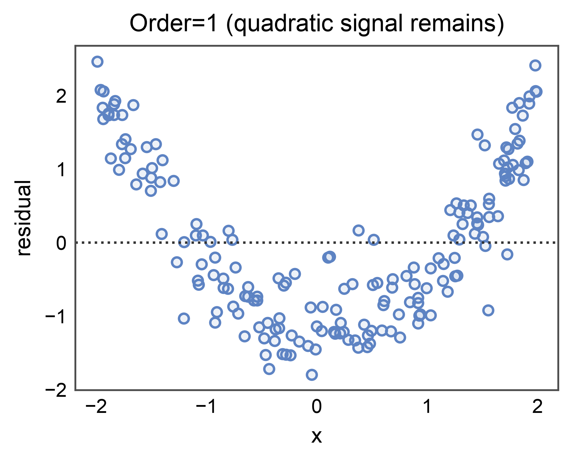
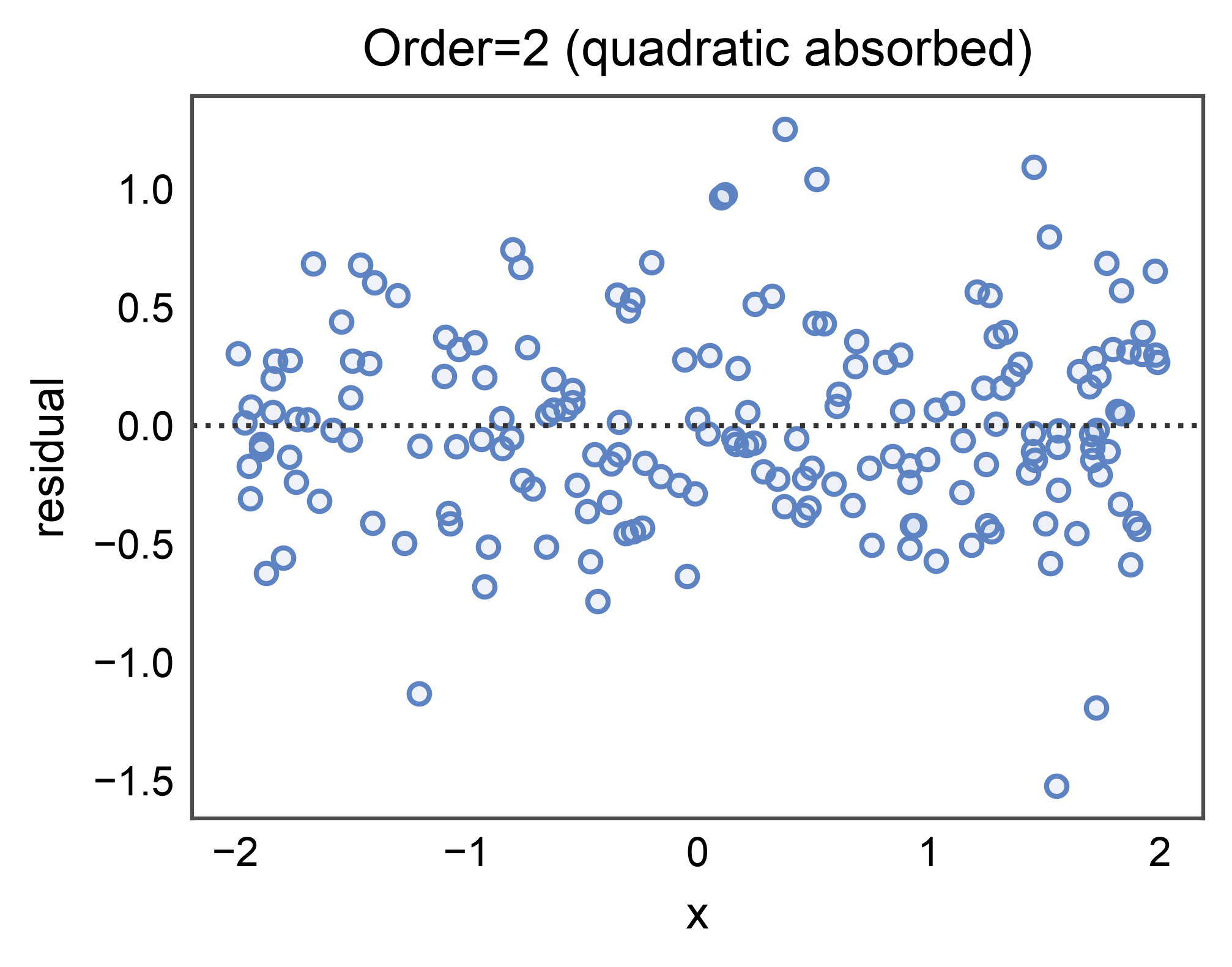
Polynomial Order (order=2)

When the underlying relationship is non-linear, a linear fit leaves systematic curvature in the residuals. Bumping order= to 2 absorbs quadratic structure — the residual cloud should look more centered on zero with no obvious bow.

rng = np.random.default_rng(0)
n = 180
x = rng.uniform(-2.0, 2.0, n)
y = 0.8 * x**2 + 0.3 * x + rng.normal(0.0, 0.4, n)
df_poly = pd.DataFrame({"x": x, "y": y})

ax = residplot(
    data=df_poly, x="x", y="y", order=1,
    title="Order=1 (quadratic signal remains)",
    xlabel="x", ylabel="residual",
)
pp.show()

ax = residplot(
    data=df_poly, x="x", y="y", order=2,
    title="Order=2 (quadratic absorbed)",
    xlabel="x", ylabel="residual",
)
pp.show()

• 
• 

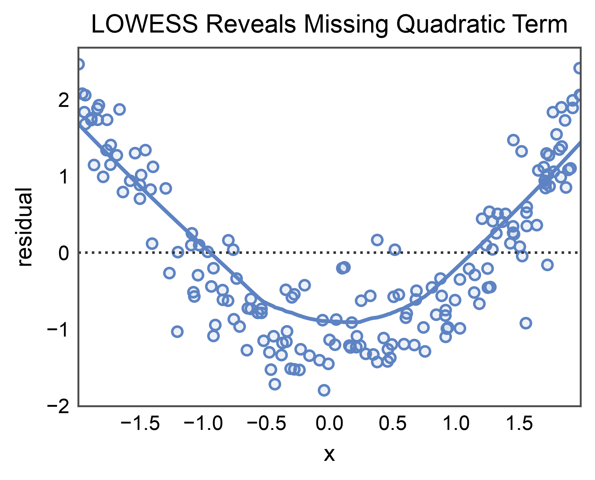
LOWESS Smoother on Residuals

lowess=True fits a nonparametric smoother on top of the residual cloud. A flat LOWESS curve is the goal; a persistent bow is evidence of unmodeled structure. Requires statsmodels (install with pip install publiplots[regression]).

try:
    import statsmodels  # noqa: F401

    ax = residplot(
        data=df_poly, x="x", y="y", order=1, lowess=True,
        title="LOWESS Reveals Missing Quadratic Term",
        xlabel="x", ylabel="residual",
    )
    pp.show()
except ImportError:
    print("statsmodels not installed; skipping LOWESS section")

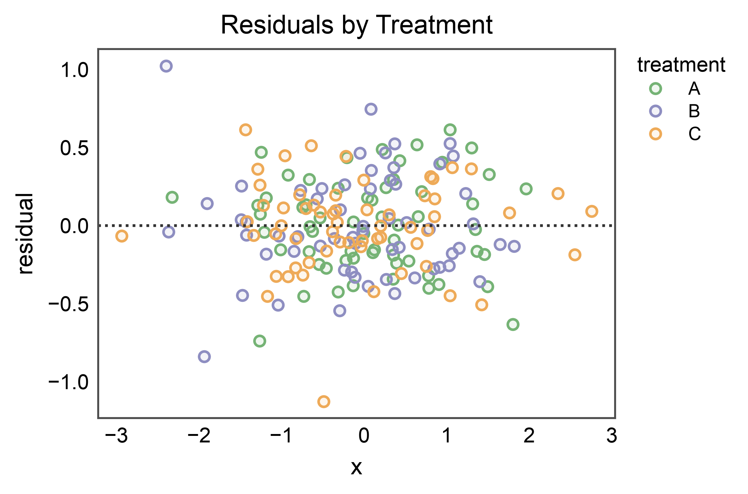
Residuals by Hue (the novelty over sns.residplot)

When hue= is passed, the data is split by level and a separate residual plot is drawn per group, each tinted by the palette. This makes it easy to compare fit quality across conditions side-by-side.

rng = np.random.default_rng(0)
n_per = 60
slopes = {"A": 1.0, "B": 0.5, "C": -0.8}
frames = []
for group, slope in slopes.items():
    xg = rng.normal(0.0, 1.0, n_per)
    yg = slope * xg + rng.normal(0.0, 0.3, n_per)
    frames.append(pd.DataFrame({"x": xg, "y": yg, "treatment": group}))
hue_df = pd.concat(frames, ignore_index=True)

ax = residplot(
    data=hue_df, x="x", y="y", hue="treatment",
    title="Residuals by Treatment",
    xlabel="x", ylabel="residual",
)
pp.show()