Regplot Examples

publiplots.regplot() wraps seaborn.regplot() with publiplots styling and adds a crucial missing feature: categorical hue= support. Seaborn’s native regplot does not accept hue; users historically had to reach for sns.lmplot (which owns its figure) to get per-group fits. pp.regplot loops over hue levels and calls sns.regplot per group onto a shared axes, preserving compatibility with publiplots.subplots() and the figure/axes layout pipeline.

import numpy as np
import pandas as pd

import publiplots as pp
from publiplots.plot.regplot import regplot

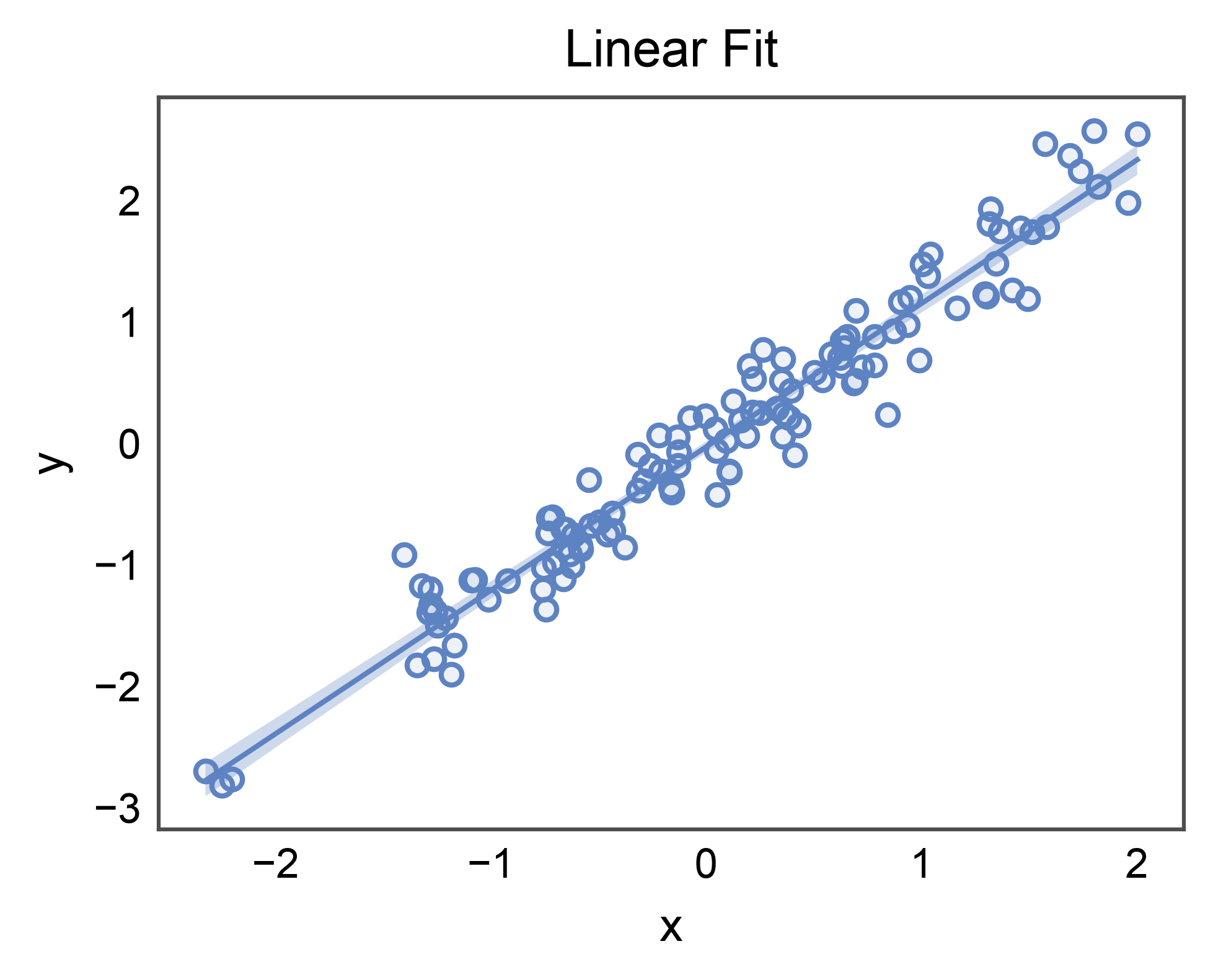
Basic Linear Fit

The un-hued case mirrors seaborn.regplot() but routes through the publiplots styling pipeline: linewidth, alpha, and edgecolor defaults come from pp.rcParams, and the figure is sized from pp.subplots(axes_size=...) rather than a figsize= kwarg.

rng = np.random.default_rng(0)
n = 120
x = rng.normal(size=n)
y = 1.2 * x + 0.25 * rng.normal(size=n)
linear_df = pd.DataFrame({"x": x, "y": y})

ax = regplot(
    data=linear_df,
    x="x",
    y="y",
    ci_kws=dict(alpha=0.3),
    title="Linear Fit",
    xlabel="x",
    ylabel="y",
)
pp.show()

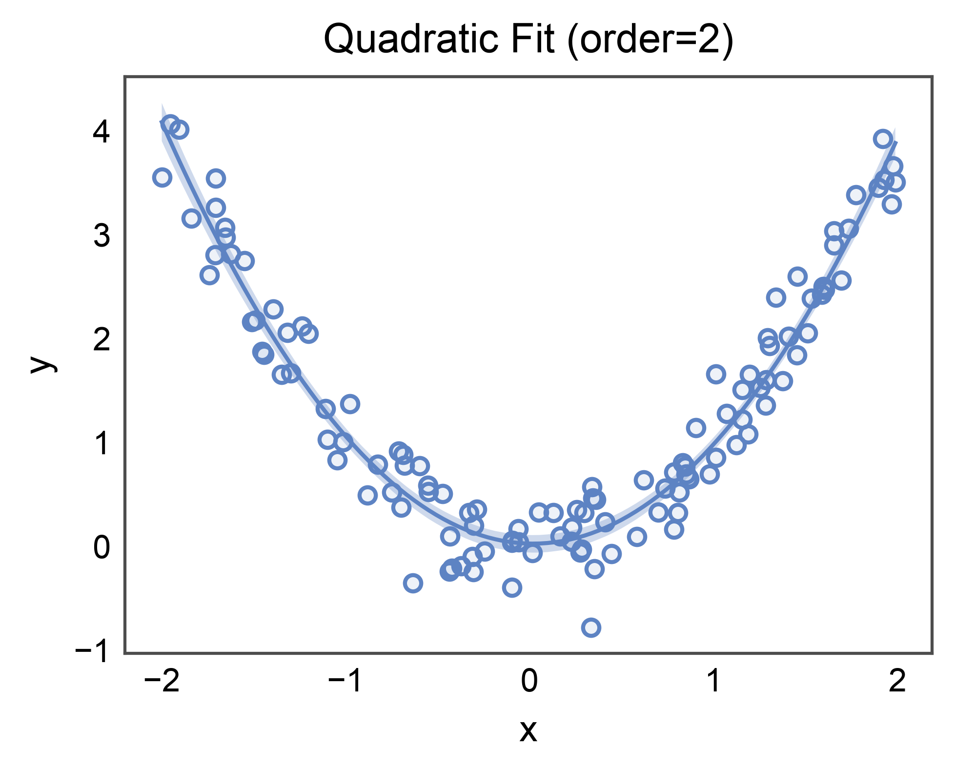
Polynomial Fit

Pass order= to fit an order-N polynomial. The CI band is bootstrapped around the curved fit the same way as for the linear case.

n = 120
x = rng.uniform(-2.0, 2.0, size=n)
y = x ** 2 + 0.3 * rng.normal(size=n)
quad_df = pd.DataFrame({"x": x, "y": y})

ax = regplot(
    data=quad_df,
    x="x",
    y="y",
    order=2,
    ci_kws=dict(alpha=0.3),
    title="Quadratic Fit (order=2)",
    xlabel="x",
    ylabel="y",
)
pp.show()

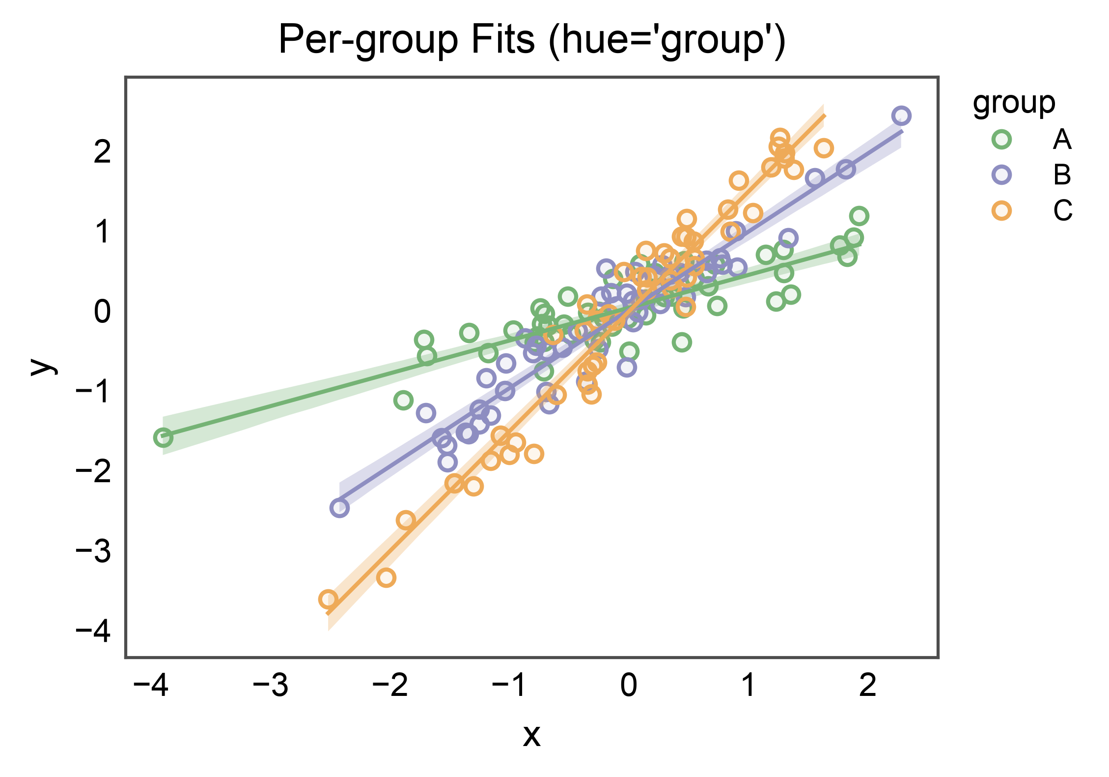
Hue’d Fits (the novelty over sns.regplot)

With hue=, pp.regplot loops over hue levels and draws one regression per group on a shared axes. Each fit carries its own CI band and scatter swatch; the palette comes from the standard publiplots palette resolver. A per-group legend is stashed automatically.

per_group = 50
rows = []
for i, g in enumerate(["A", "B", "C"]):
    gx = rng.normal(size=per_group)
    slope = 0.4 + 0.6 * i
    gy = slope * gx + 0.3 * rng.normal(size=per_group)
    rows.extend({"x": xi, "y": yi, "group": g} for xi, yi in zip(gx, gy))
hue_df = pd.DataFrame(rows)

ax = regplot(
    data=hue_df,
    x="x",
    y="y",
    hue="group",
    palette="pastel",
    ci_kws=dict(alpha=0.3),
    title="Per-group Fits (hue='group')",
    xlabel="x",
    ylabel="y",
)
pp.show()

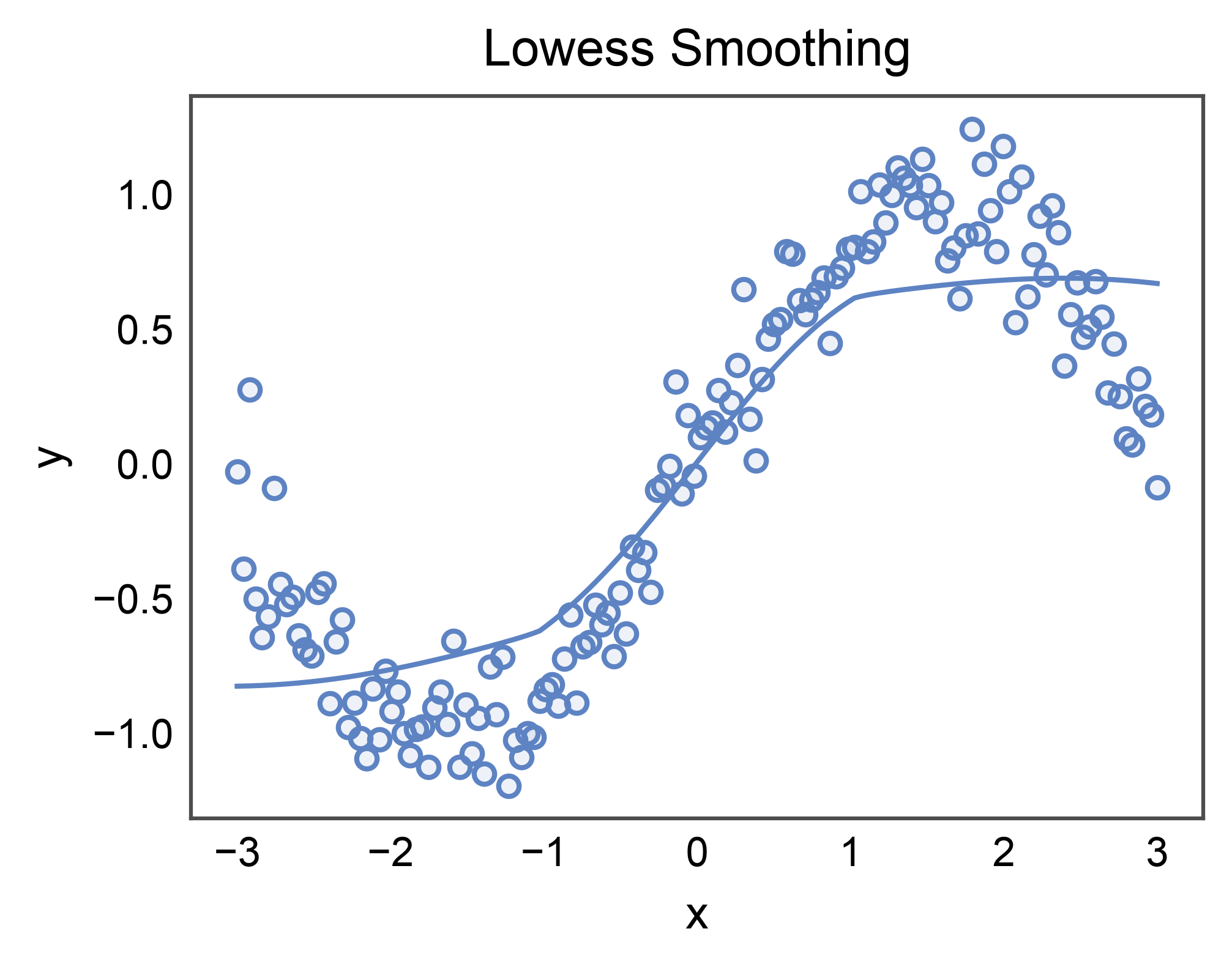
Lowess Smoothing

lowess=True fits a locally-weighted regression curve instead of an ordinary-least-squares line. Handy for data with non-parametric trends. Requires statsmodels (install with pip install publiplots[regression]).

try:
    import statsmodels  # noqa: F401

    n = 150
    x = np.linspace(-3.0, 3.0, n)
    y = np.sin(x) + 0.2 * rng.normal(size=n)
    lowess_df = pd.DataFrame({"x": x, "y": y})

    ax = regplot(
        data=lowess_df,
        x="x",
        y="y",
        lowess=True,
        ci_kws=dict(alpha=0.3),
        title="Lowess Smoothing",
        xlabel="x",
        ylabel="y",
    )
    pp.show()
except ImportError:
    print("statsmodels not installed; skipping LOWESS section")

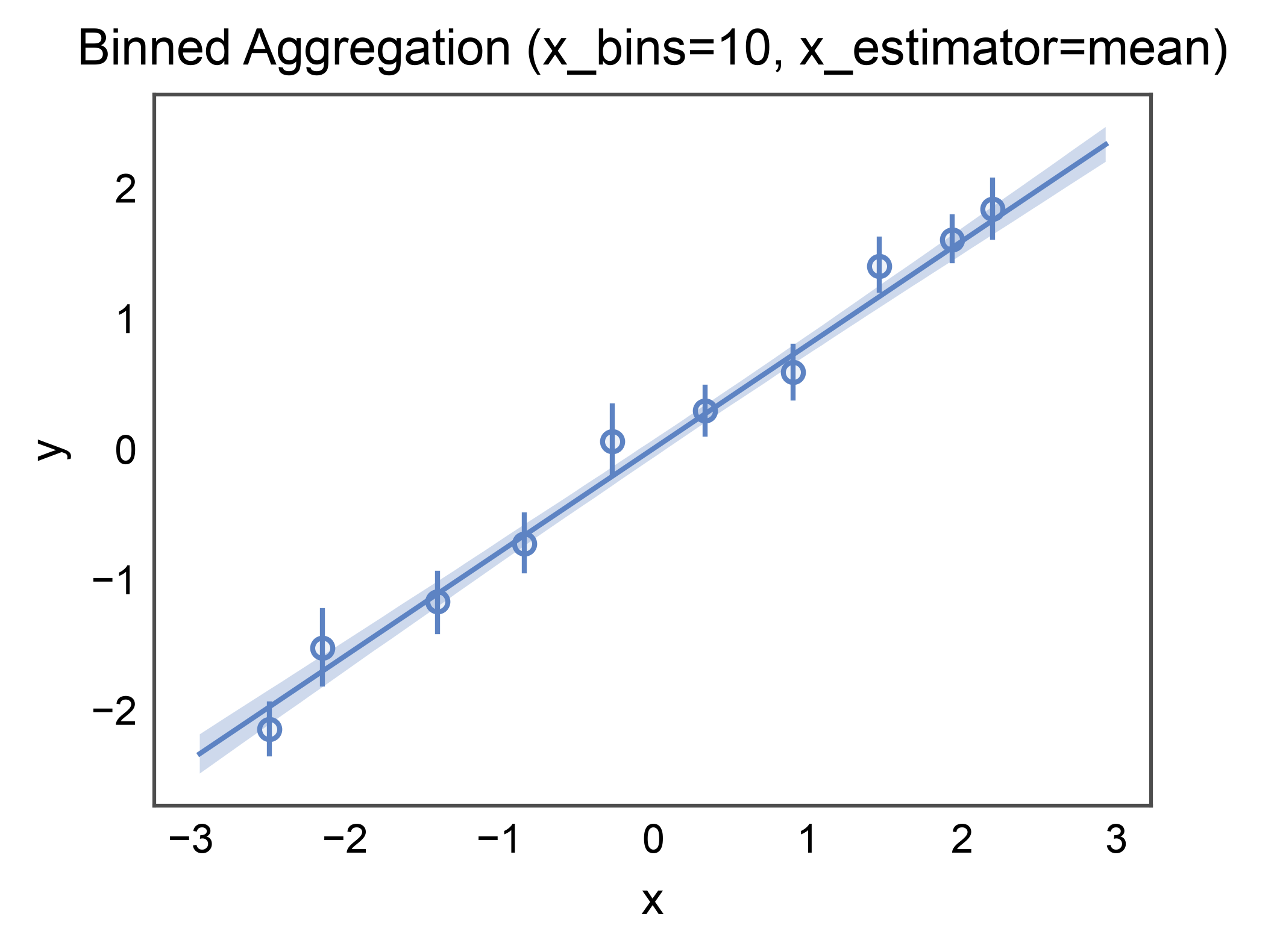
Binned Aggregation with Error Bars

x_bins= discretizes the x-axis and x_estimator= aggregates each bin’s y values. x_ci="ci" draws bootstrap error bars on each bin. Useful when the raw scatter is too dense to read but the marginal trend matters.

n = 200
x = rng.uniform(-3.0, 3.0, size=n)
y = 0.8 * x + 0.5 * rng.normal(size=n)
binned_df = pd.DataFrame({"x": x, "y": y})

ax = regplot(
    data=binned_df,
    x="x",
    y="y",
    x_bins=10,
    x_estimator=np.mean,
    ci_kws=dict(alpha=0.3),
    title="Binned Aggregation (x_bins=10, x_estimator=mean)",
    xlabel="x",
    ylabel="y",
)
pp.show()

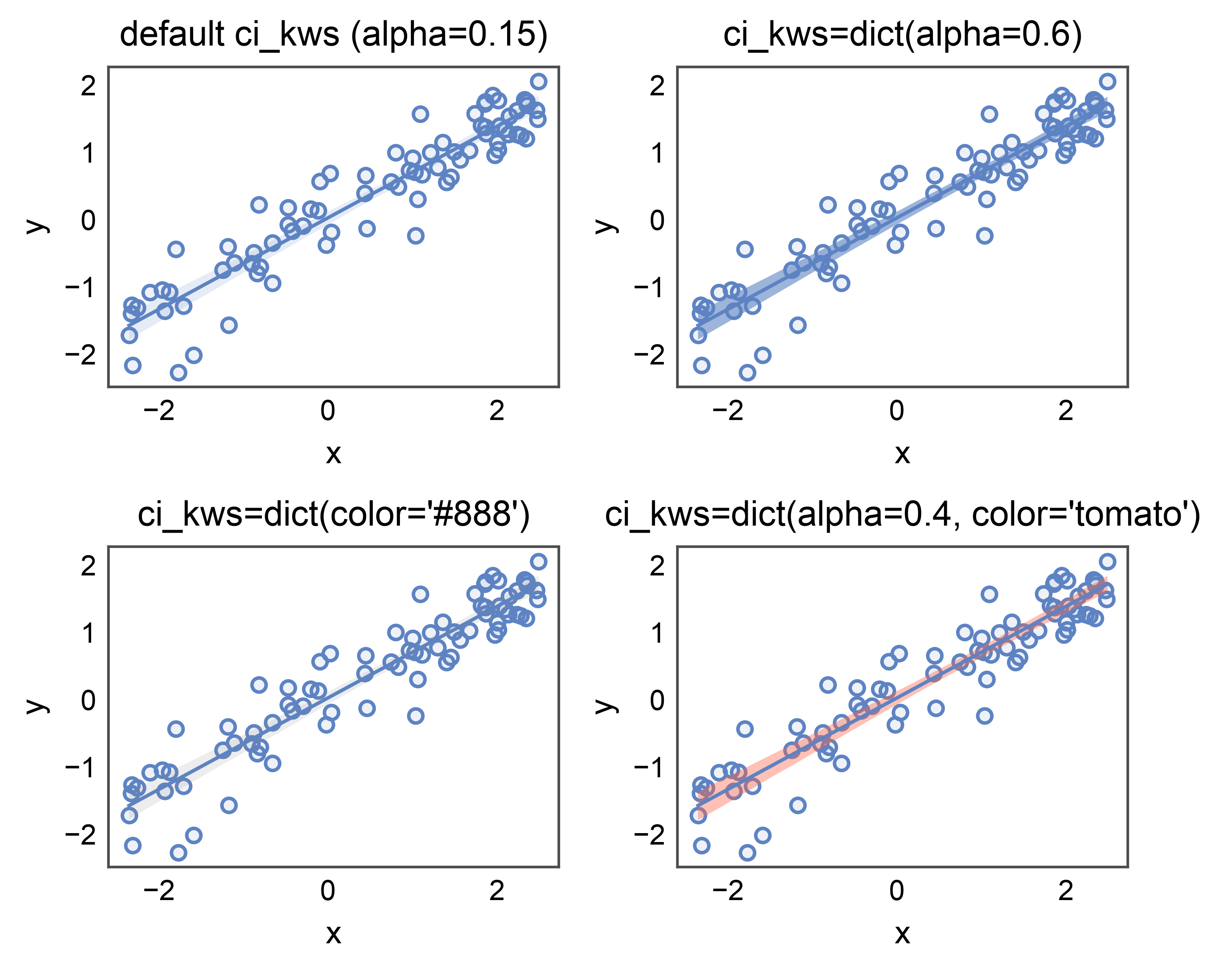
Styling the Confidence-Interval Band: ci_kws=

The CI band drawn around the fit is a separate visual layer (a FillBetweenPolyCollection) and gets its own styling bucket — ci_kws= — so the band can be tuned independently from the scatter (scatter_kws) and the regression line (line_kws).

Recognized keys:

• alpha: face alpha (default seaborn’s 0.15). Use lower for de-emphasis when overlaying multiple groups, higher for a single bold fit.

• color: face color. Defaults to the regression line color; override for accessibility / print contrast when the band needs to differ from the line.

A four-panel comparison: default → bolder alpha → recoloured band → both keys together. Same data in every panel so only the band styling moves.

n = 80
x = rng.uniform(-2.5, 2.5, n)
y = 0.7 * x + 0.4 * rng.normal(size=n)
ci_df = pd.DataFrame({"x": x, "y": y})

fig, axes = pp.subplots(2, 2, axes_size=(45, 32))
regplot(data=ci_df, x="x", y="y", ax=axes[0, 0],
        title="default ci_kws (alpha=0.15)")
regplot(data=ci_df, x="x", y="y", ci_kws=dict(alpha=0.6), ax=axes[0, 1],
        title="ci_kws=dict(alpha=0.6)")
regplot(data=ci_df, x="x", y="y", ci_kws=dict(color="#888"), ax=axes[1, 0],
        title="ci_kws=dict(color='#888')")
regplot(data=ci_df, x="x", y="y", ci_kws=dict(alpha=0.4, color="tomato"),
        ax=axes[1, 1], title="ci_kws=dict(alpha=0.4, color='tomato')")
pp.show()

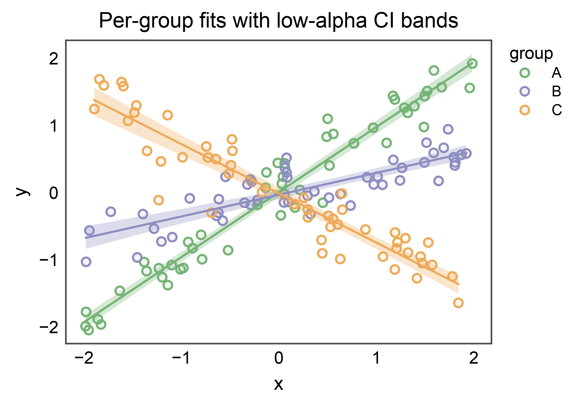
ci_kws with Hue: De-emphasize Bands When Overlaying Groups

When several regressions share an axes, full-strength CI bands stack into mud. A lower ci_kws['alpha'] (e.g. 0.3) pushes the bands into the visual background while the per-group lines and scatter remain crisp. Each band still inherits its group’s palette color — ci_kws only overrides the keys you set.

rng2 = np.random.default_rng(7)
rows = []
for slope, g in zip((1.0, 0.3, -0.7), ("A", "B", "C")):
    xs = rng2.uniform(-2, 2, 50)
    ys = slope * xs + 0.3 * rng2.normal(size=50)
    rows.extend({"x": xi, "y": yi, "group": g} for xi, yi in zip(xs, ys))
hue_groups = pd.DataFrame(rows)

ax = regplot(
    data=hue_groups,
    x="x",
    y="y",
    hue="group",
    palette="pastel",
    ci_kws=dict(alpha=0.3),
    title="Per-group fits with low-alpha CI bands",
    xlabel="x",
    ylabel="y",
)
pp.show()