Heatmap Examples

This example demonstrates the heatmap capabilities in PubliPlots, including standard heatmaps, dot heatmaps, clustered heatmaps, and complex heatmaps with margin plots.

import publiplots as pp
import pandas as pd
import numpy as np
import matplotlib.pyplot as plt

# Set style
pp.set_notebook_style()

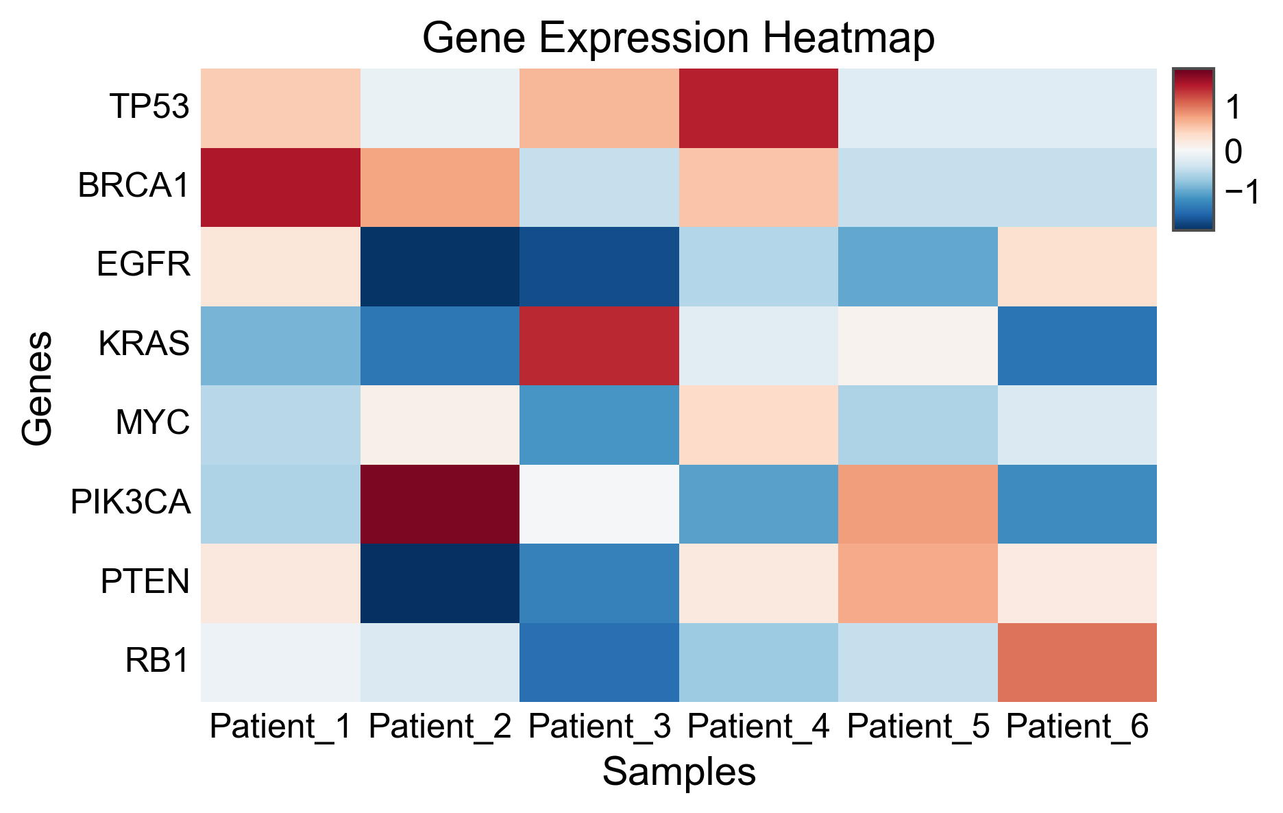
Simple Heatmap (Wide Format)

Create a basic heatmap from a matrix DataFrame.

# Create sample expression matrix
np.random.seed(42)
genes = ['TP53', 'BRCA1', 'EGFR', 'KRAS', 'MYC', 'PIK3CA', 'PTEN', 'RB1']
samples = ['Patient_' + str(i) for i in range(1, 7)]

expression_matrix = pd.DataFrame(
    np.random.randn(len(genes), len(samples)),
    index=genes,
    columns=samples
)

# Create heatmap with diverging colormap centered at 0
fig, ax = pp.heatmap(
    expression_matrix,
    cmap='RdBu_r',
    center=0,
    title='Gene Expression Heatmap',
    xlabel='Samples',
    ylabel='Genes',
)
plt.show()

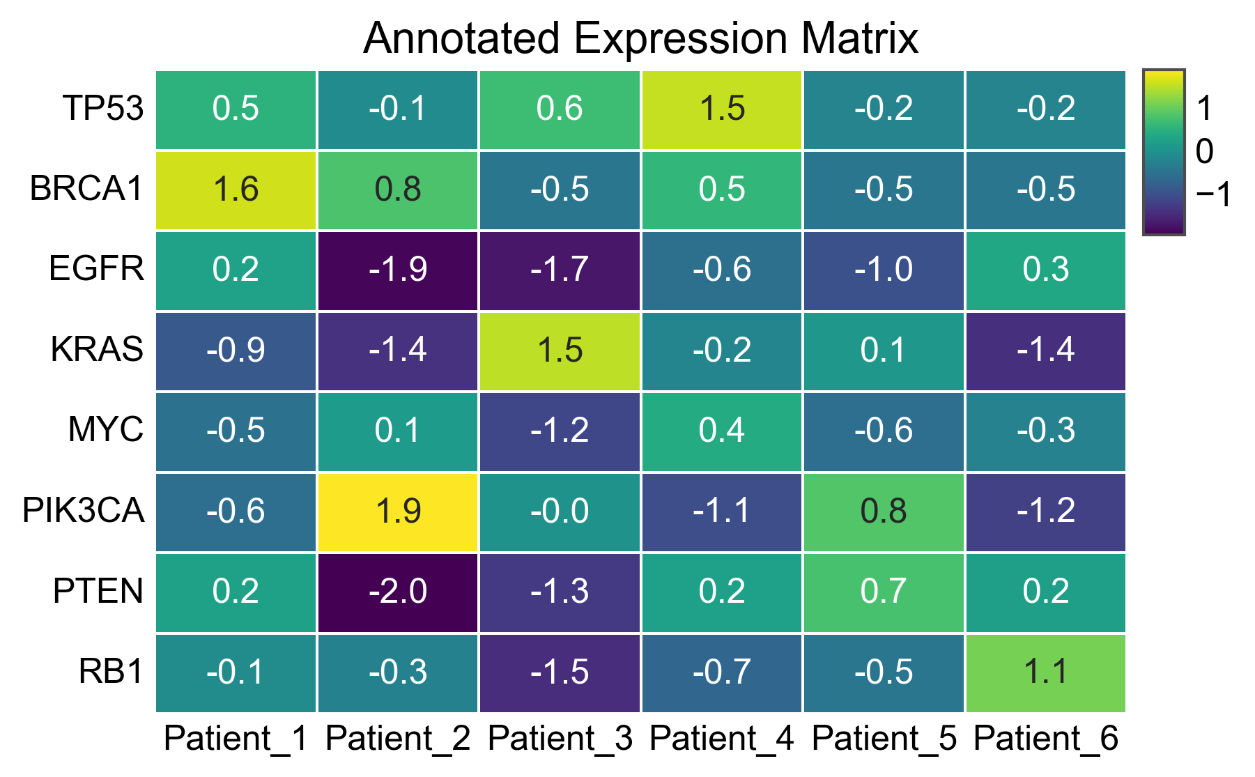
Annotated Heatmap

Display values inside each cell.

fig, ax = pp.heatmap(
    expression_matrix,
    cmap='viridis',
    annot=True,
    fmt='.1f',
    linewidths=0.5,
    linecolor='white',
    title='Annotated Expression Matrix',
)
plt.show()

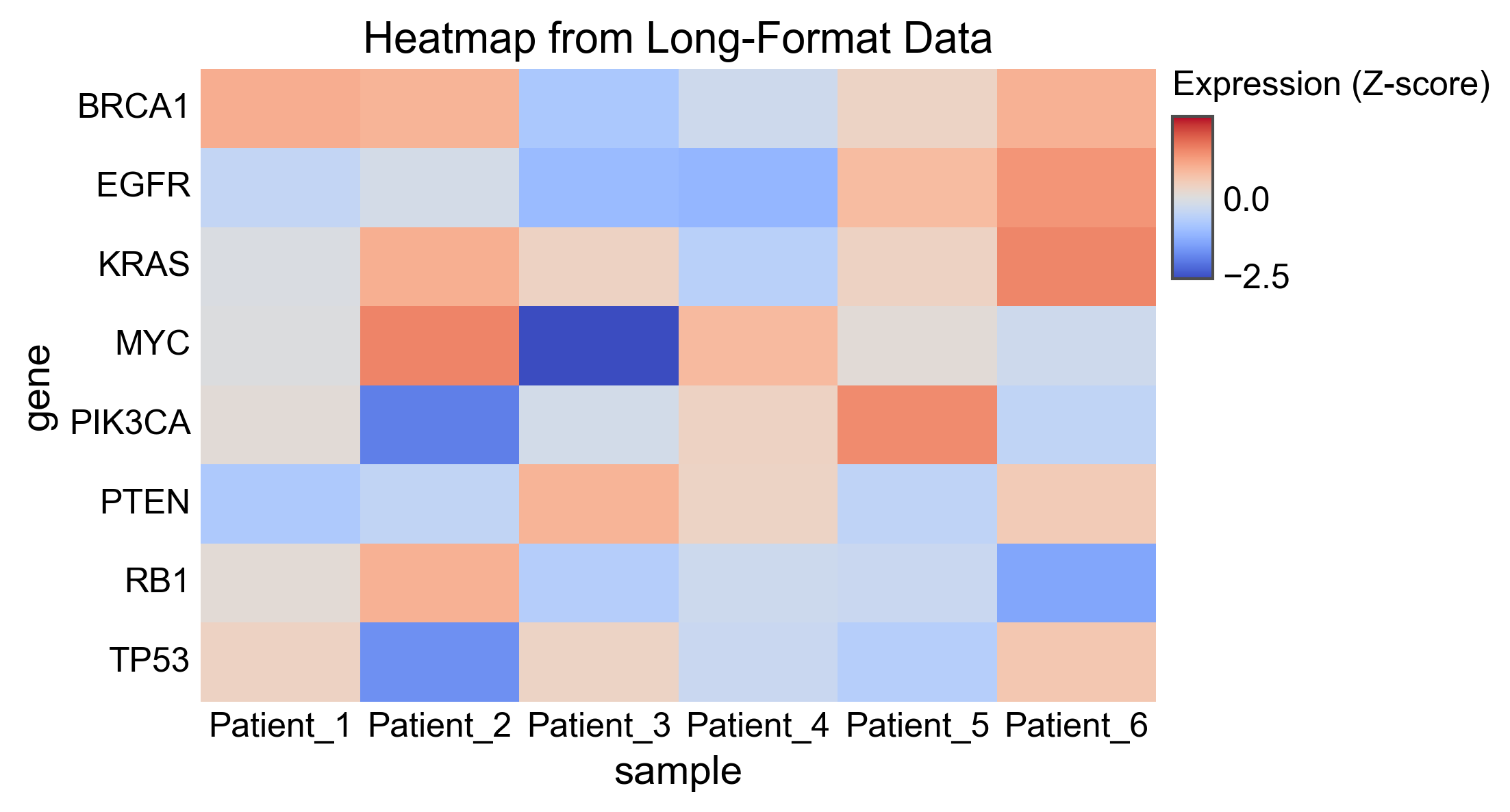
Heatmap from Long-Format Data

Use x, y, value parameters for tidy data.

# Create long-format data
long_data = []
for gene in genes:
    for sample in samples:
        long_data.append({
            'gene': gene,
            'sample': sample,
            'expression': np.random.randn(),
        })
long_df = pd.DataFrame(long_data)

fig, ax = pp.heatmap(
    long_df,
    x='sample',
    y='gene',
    value='expression',
    cmap='coolwarm',
    center=0,
    title='Heatmap from Long-Format Data',
    legend_kws={'value_label': 'Expression (Z-score)'},
)
plt.show()

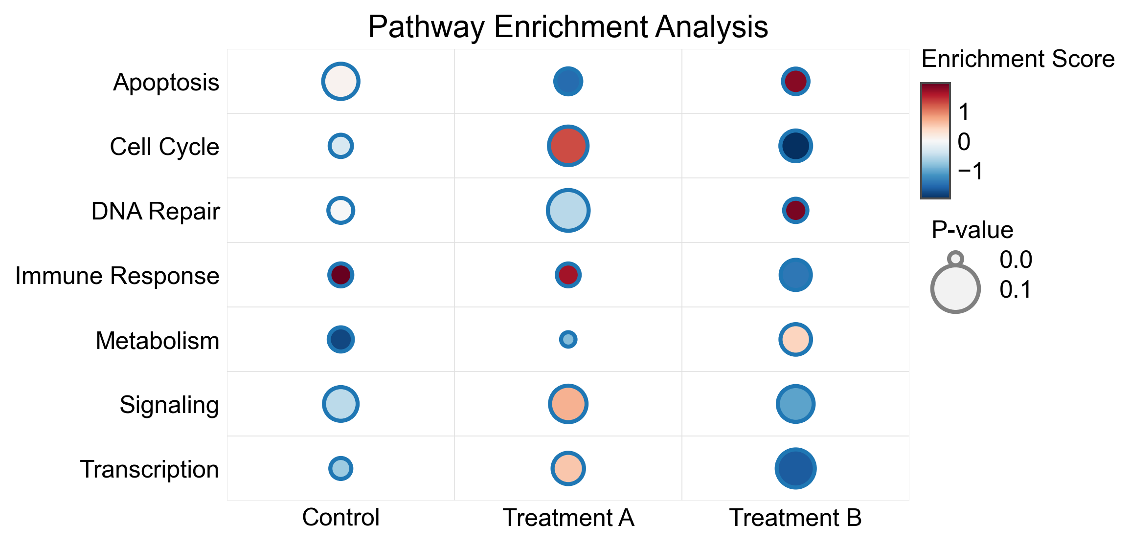
Dot Heatmap (Bubble Plot)

Use size encoding for an additional variable, perfect for enrichment analysis or differential expression results.

# Create enrichment-style data
pathways = ['Cell Cycle', 'Apoptosis', 'DNA Repair', 'Metabolism',
            'Immune Response', 'Signaling', 'Transcription']
conditions = ['Treatment A', 'Treatment B', 'Control']

enrichment_data = []
for pathway in pathways:
    for condition in conditions:
        enrichment_data.append({
            'pathway': pathway,
            'condition': condition,
            'enrichment': np.random.uniform(-2, 2),
            'pvalue': np.random.uniform(0.001, 0.1),
        })
enrichment_df = pd.DataFrame(enrichment_data)

fig, ax = pp.heatmap(
    enrichment_df,
    x='condition',
    y='pathway',
    value='enrichment',
    size='pvalue',
    cmap='RdBu_r',
    center=0,
    sizes=(50, 400),
    title='Pathway Enrichment Analysis',
    legend_kws={
        'value_label': 'Enrichment Score',
        'size_label': 'P-value',
    },
)
plt.show()

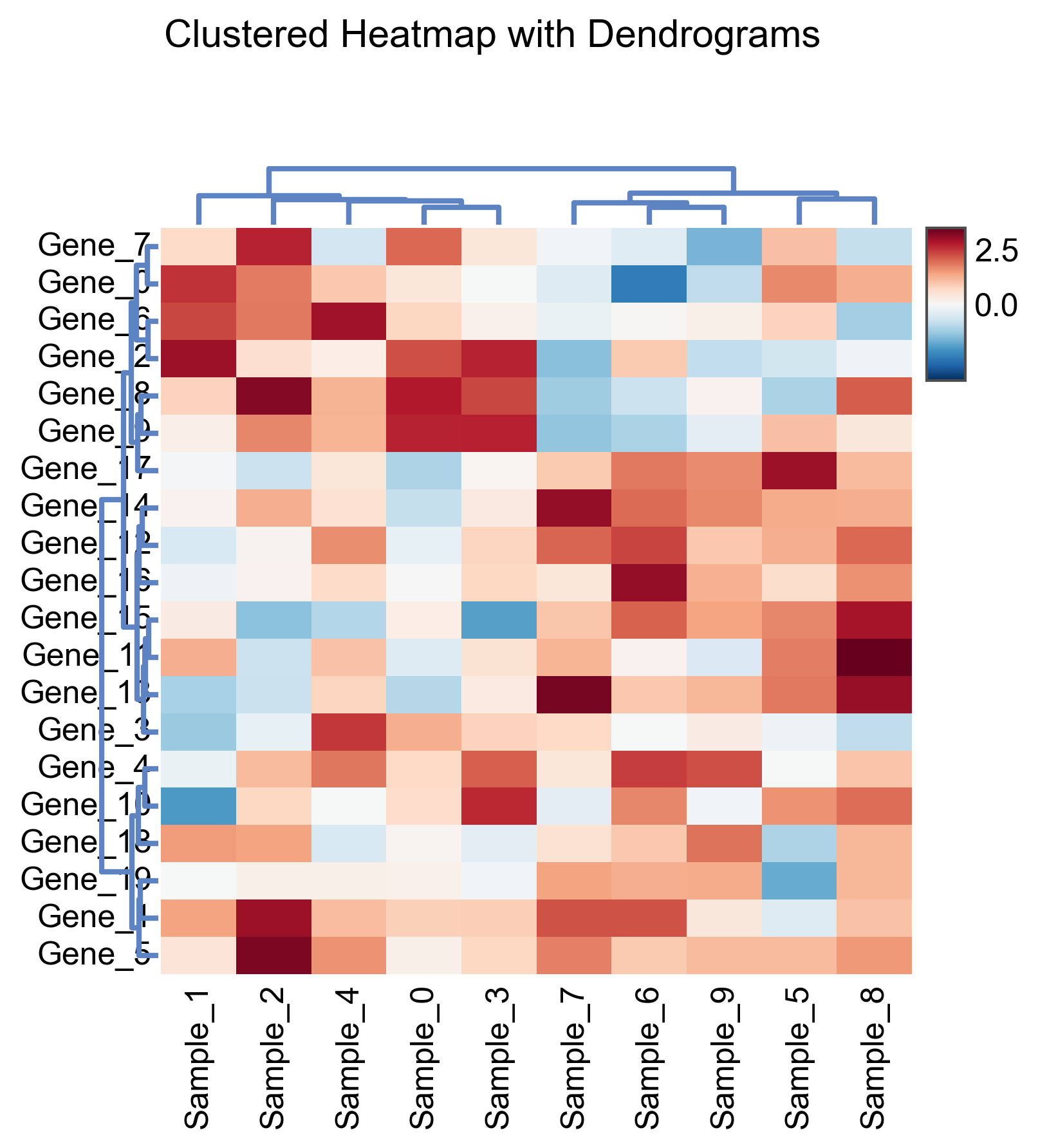
Clustered Heatmap

Use complex_heatmap with clustering to automatically reorder rows and columns and add dendrograms.

# Create larger expression matrix for clustering
np.random.seed(123)
n_genes = 20
n_samples = 10

# Create data with some structure for interesting clustering
cluster_matrix = pd.DataFrame(
    np.random.randn(n_genes, n_samples),
    index=['Gene_' + str(i) for i in range(n_genes)],
    columns=['Sample_' + str(i) for i in range(n_samples)]
)
# Add some cluster structure
cluster_matrix.iloc[:10, :5] += 1.5
cluster_matrix.iloc[10:, 5:] += 1.5

fig, axes = (
    pp.complex_heatmap(
        cluster_matrix,
        cmap='RdBu_r',
        center=0,
        row_cluster=True,
        col_cluster=True,
        figsize=(5, 5),
    )
    .build()
)
plt.suptitle('Clustered Heatmap with Dendrograms', y=1.02)
plt.show()

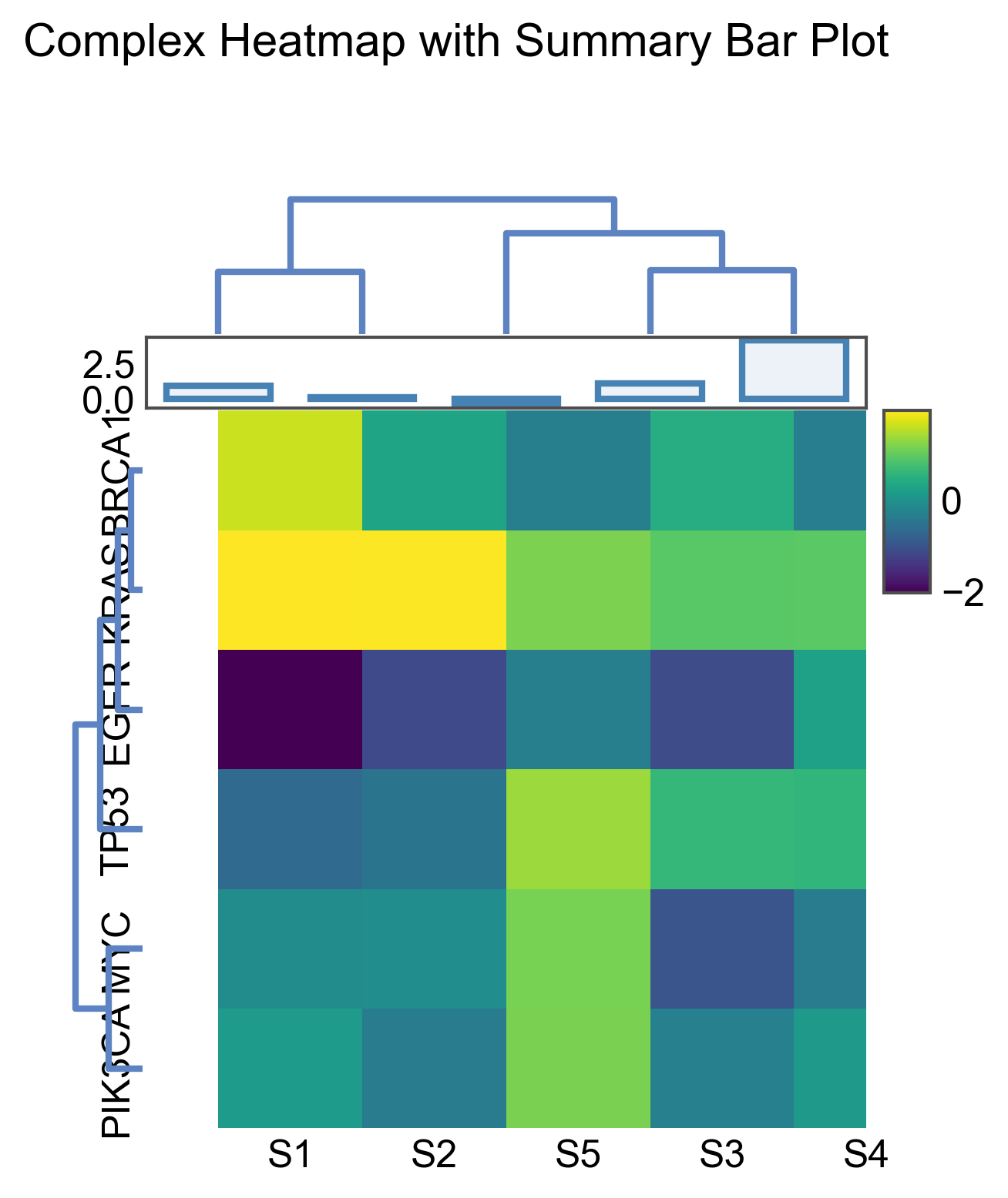
Complex Heatmap with Margin Plots

Add bar plots to the margins to show summary statistics.

# Create expression data
np.random.seed(456)
genes = ['TP53', 'BRCA1', 'EGFR', 'KRAS', 'MYC', 'PIK3CA']
samples = ['S1', 'S2', 'S3', 'S4', 'S5']

expr_matrix = pd.DataFrame(
    np.random.randn(len(genes), len(samples)),
    index=genes,
    columns=samples
)

# Create summary data for margins
# Column (sample) summaries - total expression per sample
col_summary = pd.DataFrame({
    'sample': samples,
    'total': expr_matrix.sum(axis=0).values,
})

# Row (gene) summaries - mean expression per gene
row_summary = pd.DataFrame({
    'gene': genes,
    'mean': expr_matrix.mean(axis=1).values,
})

fig, axes = (
    pp.complex_heatmap(
        expr_matrix,
        cmap='viridis',
        figsize=(4, 4),
        row_cluster=True,
        col_cluster=True,
    )
    .add_top(
        pp.barplot,
        data=col_summary,
        x='sample',
        y='total',
        height=20,
        color='steelblue',
    )
    .build()
)
plt.suptitle('Complex Heatmap with Summary Bar Plot', y=1.02)
plt.show()

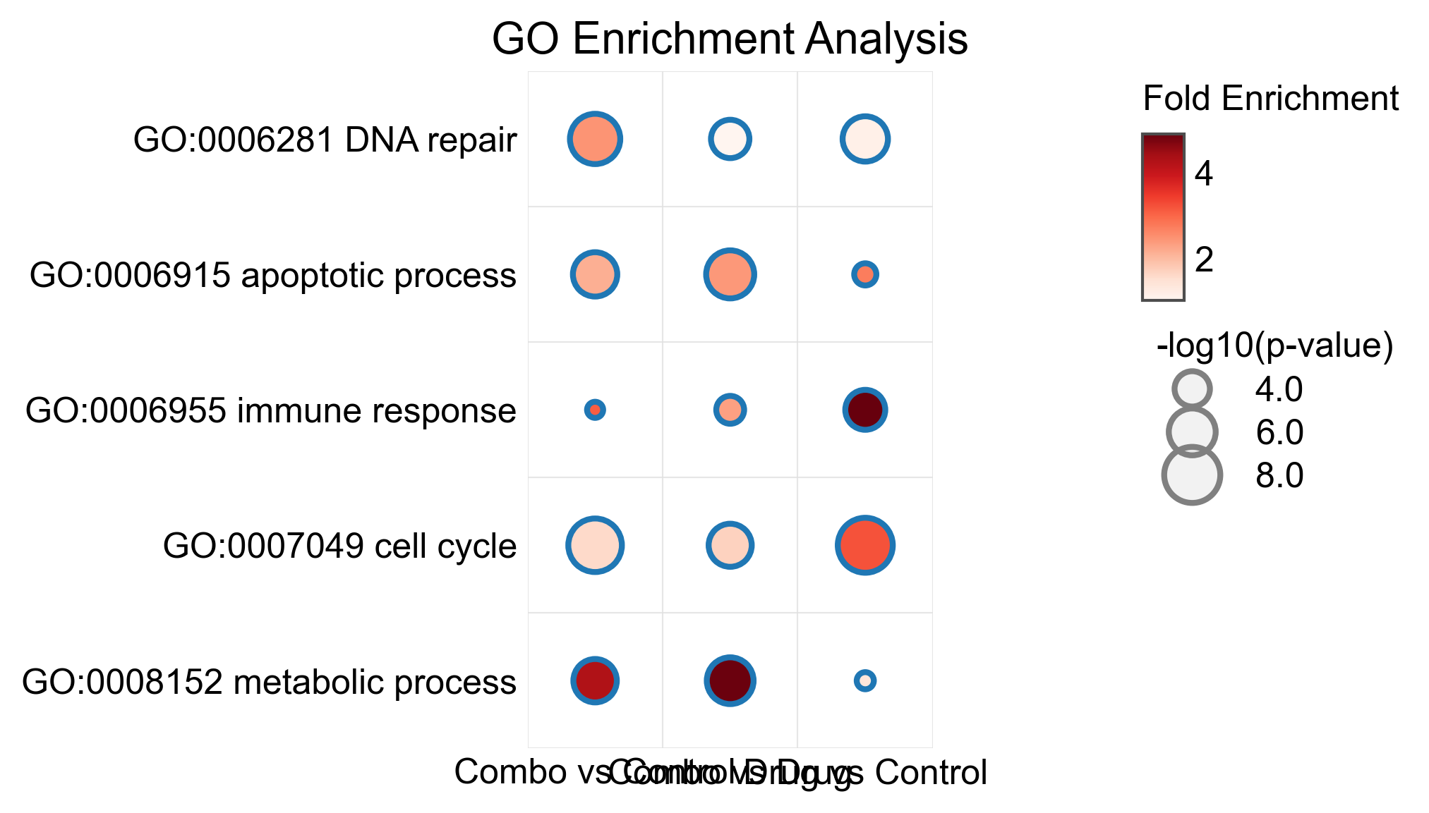
Dot Heatmap for GO Enrichment

A common visualization for gene ontology enrichment results.

# Simulated GO enrichment results
go_terms = [
    'GO:0006915 apoptotic process',
    'GO:0007049 cell cycle',
    'GO:0006281 DNA repair',
    'GO:0008152 metabolic process',
    'GO:0006955 immune response',
]
comparisons = ['Drug vs Control', 'Combo vs Control', 'Combo vs Drug']

go_data = []
for term in go_terms:
    for comp in comparisons:
        go_data.append({
            'GO_term': term,
            'comparison': comp,
            'fold_enrichment': np.random.uniform(1, 5),
            'neg_log_pvalue': np.random.uniform(1, 10),
        })
go_df = pd.DataFrame(go_data)

fig, ax = pp.heatmap(
    go_df,
    x='comparison',
    y='GO_term',
    value='fold_enrichment',
    size='neg_log_pvalue',
    cmap='Reds',
    sizes=(30, 350),
    title='GO Enrichment Analysis',
    legend_kws={
        'value_label': 'Fold Enrichment',
        'size_label': '-log10(p-value)',
    },
)
plt.tight_layout()
plt.show()

/home/runner/work/publiplots/publiplots/examples/plots/plot_13_heatmap.py:253: UserWarning: This figure includes Axes that are not compatible with tight_layout, so results might be incorrect.
  plt.tight_layout()

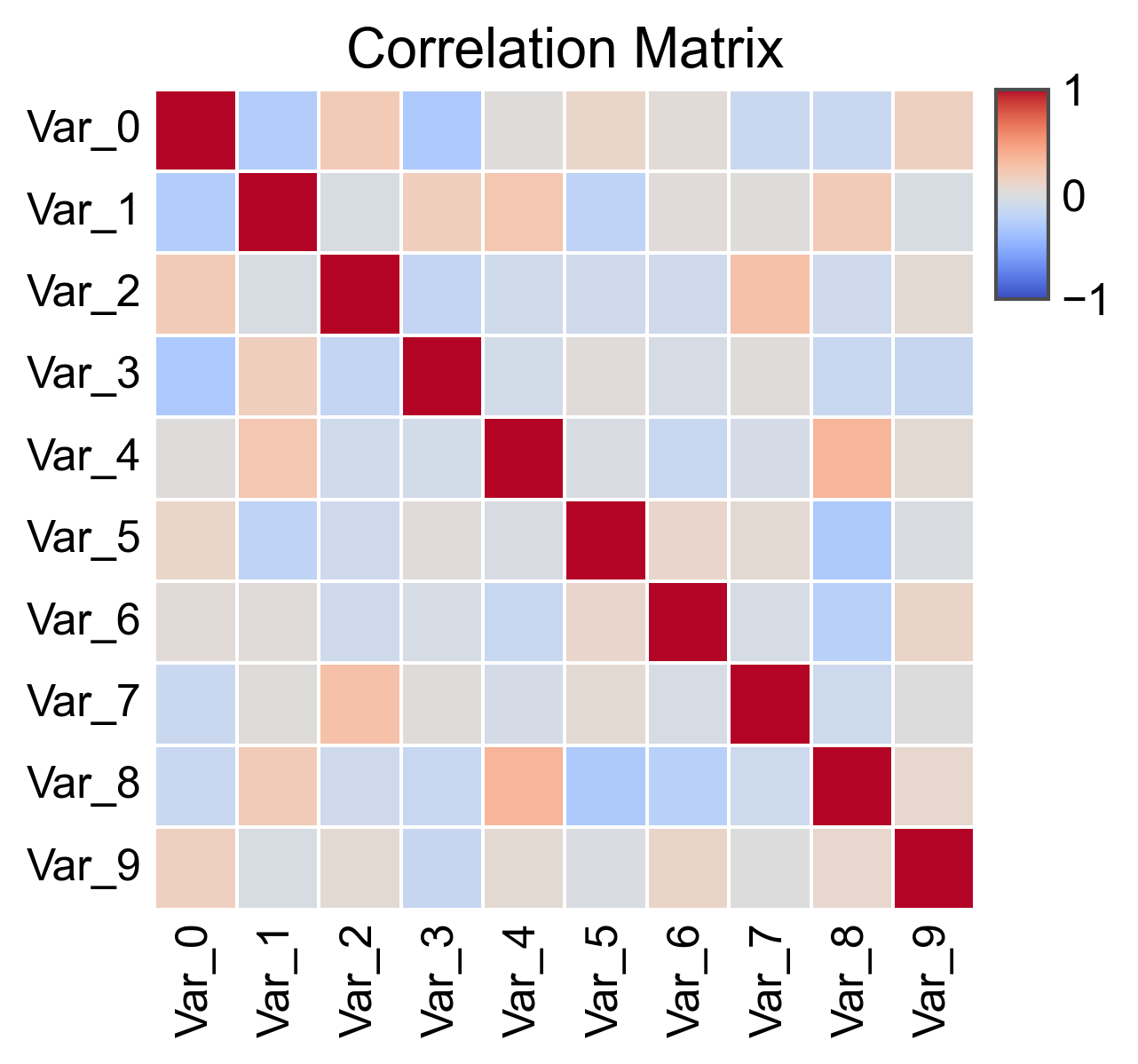
Square Heatmap

Force square cells for correlation matrices or similar data.

# Create correlation matrix
corr_data = pd.DataFrame(
    np.random.randn(10, 50)
).T.corr()
corr_data.index = ['Var_' + str(i) for i in range(10)]
corr_data.columns = corr_data.index

fig, ax = pp.heatmap(
    corr_data,
    cmap='coolwarm',
    center=0,
    vmin=-1,
    vmax=1,
    square=True,
    linewidths=0.5,
    title='Correlation Matrix',
)
plt.show()

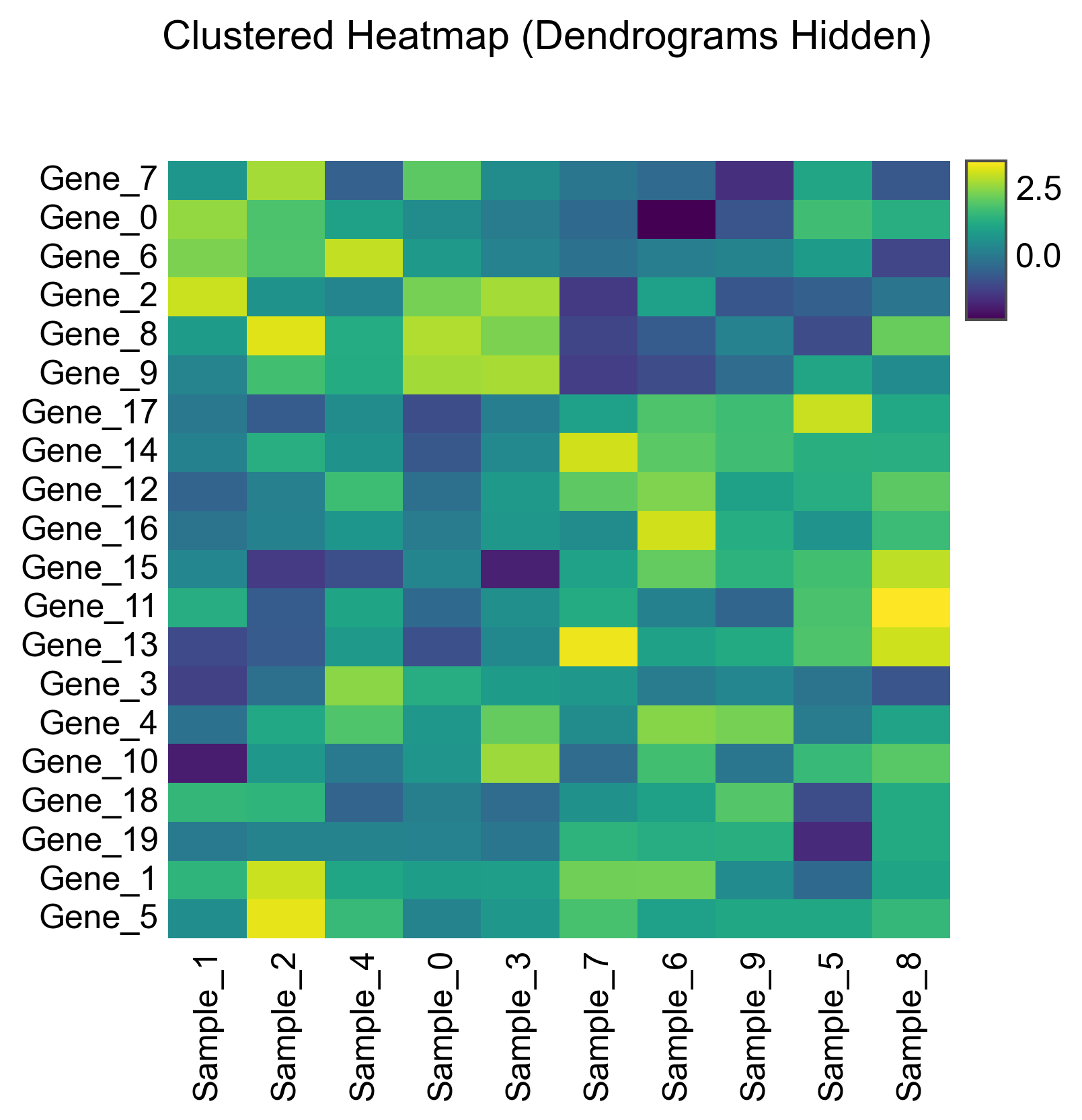
Complex Heatmap Without Dendrograms

Cluster the data but hide the dendrograms.

fig, axes = (
    pp.complex_heatmap(
        cluster_matrix,
        cmap='viridis',
        row_cluster=True,
        col_cluster=True,
        row_dendrogram=False,  # Hide row dendrogram
        col_dendrogram=False,  # Hide column dendrogram
        figsize=(5, 5),
    )
    .build()
)
plt.suptitle('Clustered Heatmap (Dendrograms Hidden)', y=1.02)
plt.show()