Hatch Pattern Examples

This example demonstrates hatch pattern functionality in PubliPlots. Hatch patterns are useful for creating black-and-white publication-ready figures that are distinguishable without relying on color.

import publiplots as pp
import pandas as pd
import numpy as np
import matplotlib.pyplot as plt

# Set style
pp.set_notebook_style()

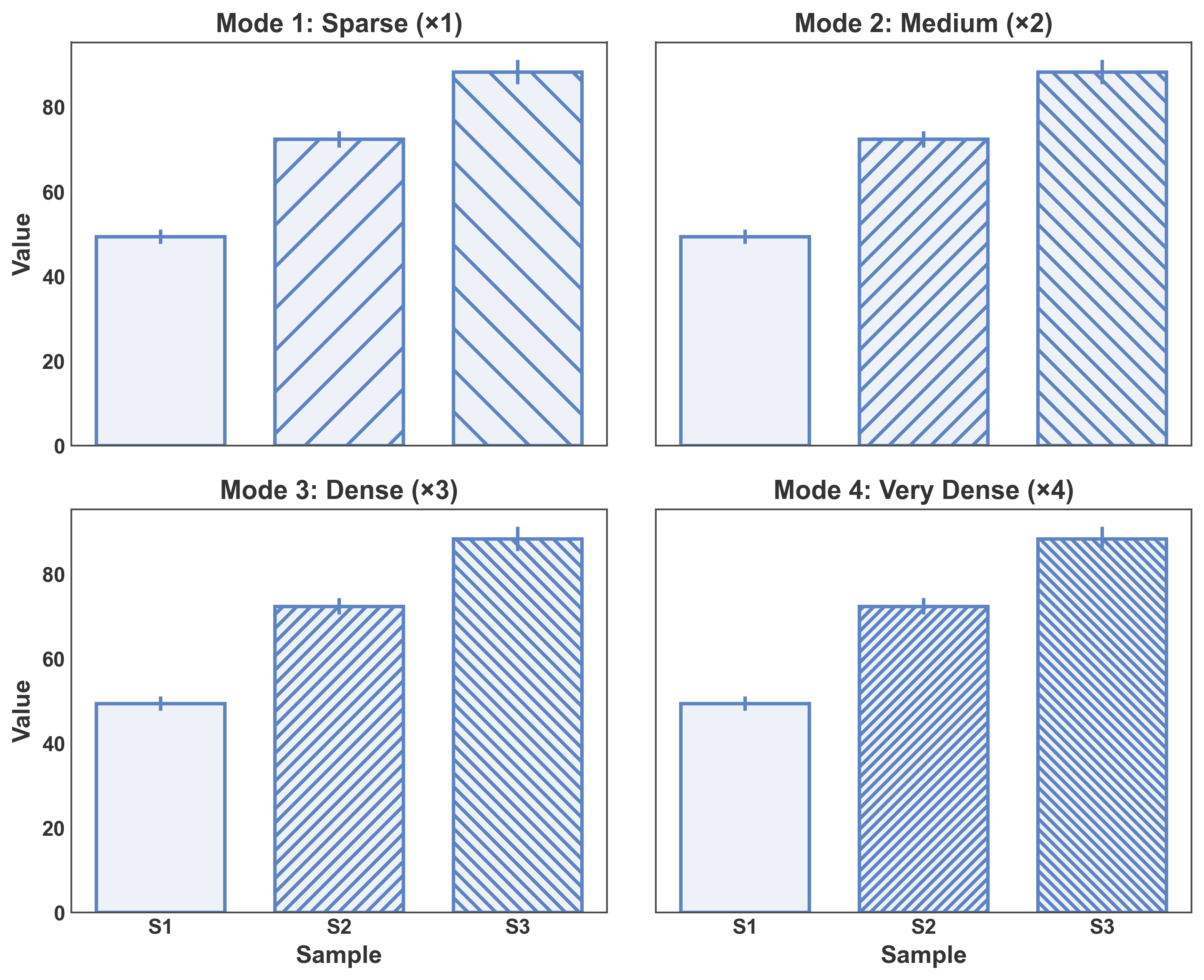
Understanding Hatch Modes

PubliPlots supports multiple hatch pattern density modes: - Mode 1 (default): Sparse patterns (base × 1, e.g., ‘/’) - Mode 2: Medium density (base × 2, e.g., ‘//’) - Mode 3: Dense patterns (base × 3, e.g., ‘///’) - Mode 4: Very dense (base × 4, e.g., ‘////’)

# Create sample data
np.random.seed(333)
hatch_mode_data = pd.DataFrame({
    'sample': np.repeat(['S1', 'S2', 'S3'], 10),
    'value': np.concatenate([
        np.random.normal(50, 5, 10),
        np.random.normal(70, 6, 10),
        np.random.normal(90, 7, 10),
    ])
})

# Create figure comparing different hatch modes
fig, axes = plt.subplots(2, 2, figsize=(10, 8), sharex=True, sharey=True)
kwargs = dict(
    data=hatch_mode_data,
    x='sample',
    y='value',
    hatch='sample',
    xlabel='Sample',
    ylabel='Value',
    color='#5D83C3',
    errorbar='se',
)

# Mode 1 (sparse)
pp.set_hatch_mode(1)
pp.barplot(
    **kwargs,
    title=f'Mode 1: Sparse (×{pp.get_hatch_mode()})',
    ax=axes[0, 0]
)

# Mode 2 (medium)
pp.set_hatch_mode(2)
pp.barplot(
    **kwargs,
    title=f'Mode 2: Medium (×{pp.get_hatch_mode()})',
    ax=axes[0, 1]
)

# Mode 3 (dense)
pp.set_hatch_mode(3)
pp.barplot(
    **kwargs,
    title=f'Mode 3: Dense (×{pp.get_hatch_mode()})',
    ax=axes[1, 0]
)

# Mode 4 (very dense)
pp.set_hatch_mode(4)
pp.barplot(
    **kwargs,
    title=f'Mode 4: Very Dense (×{pp.get_hatch_mode()})',
    ax=axes[1, 1]
)

plt.tight_layout()
plt.show()

# Reset to default
pp.set_hatch_mode()

Available Hatch Patterns

View all available hatch patterns for the current mode.

print("Available hatch patterns for mode 2:")
pp.set_hatch_mode(2)
pp.list_hatch_patterns()

# Reset to default
pp.set_hatch_mode()

Available hatch patterns for mode 2:
Hatch Patterns (Mode 2):
  0: '' (no hatch)
  1: '//'
  2: '\\'
  3: '..'
  4: '||'
  5: '--'
  6: '++'
  7: 'xx'

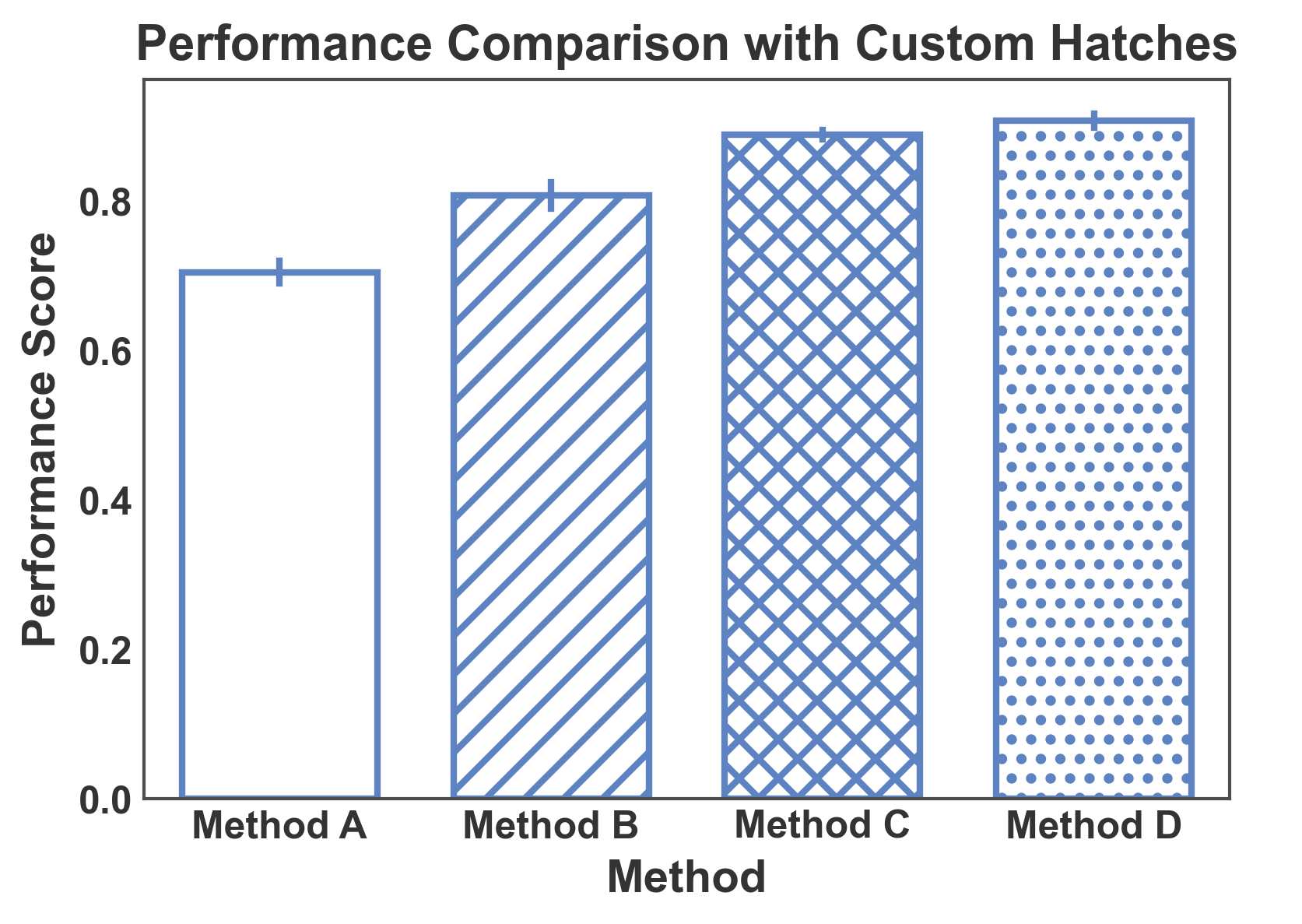
Custom Hatch Mapping

Use custom hatch patterns for specific categories.

# Create comparison data
np.random.seed(444)
method_data = pd.DataFrame({
    'method': np.repeat(['Method A', 'Method B', 'Method C', 'Method D'], 12),
    'performance': np.concatenate([
        np.random.normal(0.70, 0.06, 12),
        np.random.normal(0.82, 0.05, 12),
        np.random.normal(0.88, 0.04, 12),
        np.random.normal(0.91, 0.03, 12),
    ])
})

# Set hatch mode
pp.set_hatch_mode(2)

# Create plot with custom hatch mapping
fig, ax = pp.barplot(
    data=method_data,
    x='method',
    y='performance',
    hatch='method',
    hatch_map={
        'Method A': '',      # No hatch
        'Method B': '//',    # Diagonal lines
        'Method C': 'xx',    # Cross hatch
        'Method D': '..'     # Dots
    },
    title='Performance Comparison with Custom Hatches',
    xlabel='Method',
    ylabel='Performance Score',
    errorbar='se',
    color='#5D83C3',
    alpha=0.0,
)
plt.show()

# Reset mode
pp.set_hatch_mode()

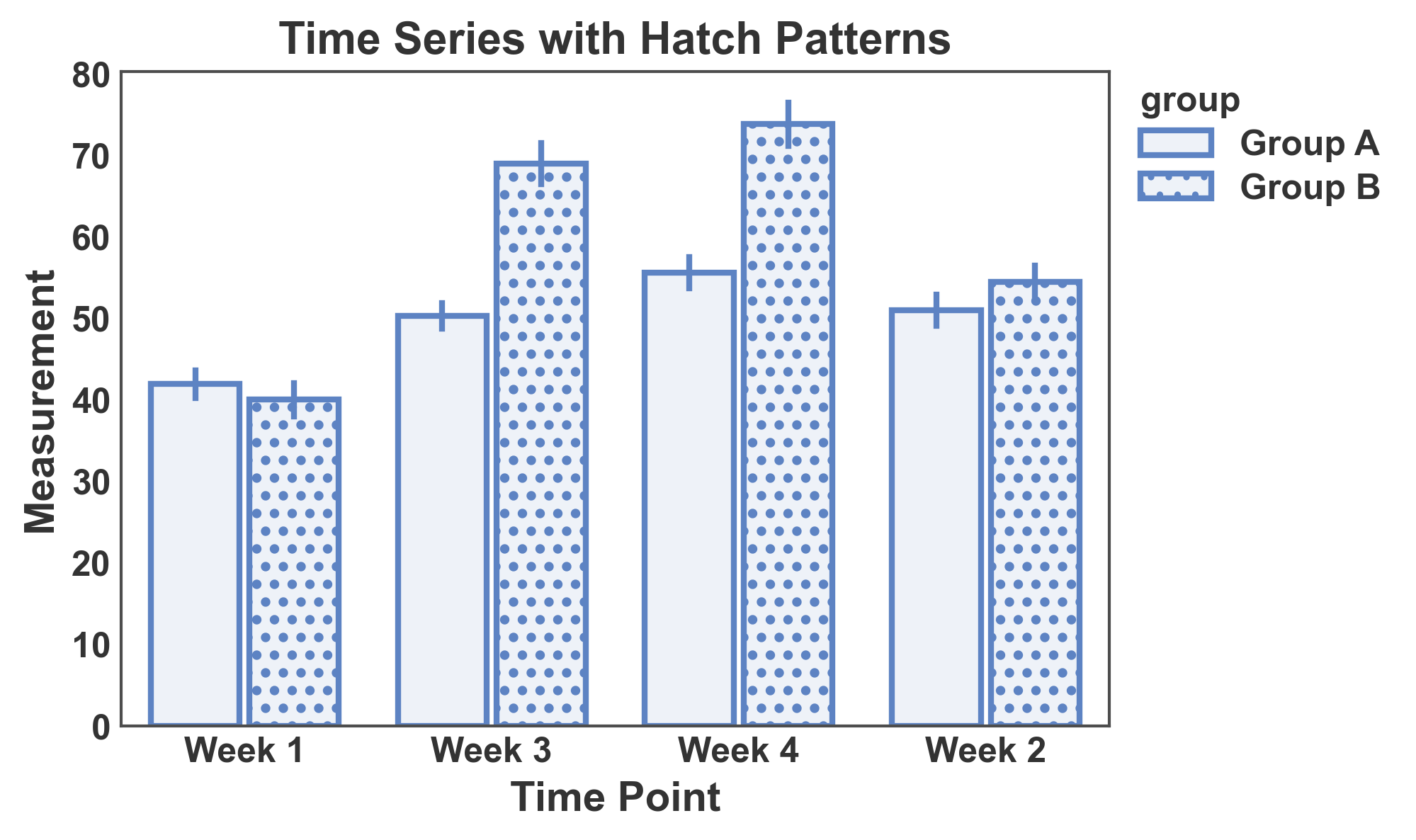
Hatch Patterns for Grouped Data

Combine hatch patterns with grouping for complex visualizations.

# Create grouped time-series data
np.random.seed(555)
timeseries_data = pd.DataFrame({
    'time': np.repeat(['Week 1', 'Week 2', 'Week 3', 'Week 4'], 24),
    'group': np.tile(np.repeat(['Group A', 'Group B'], 12), 4),
    'value': np.concatenate([
        # Week 1
        np.random.normal(40, 6, 12),   # Group A
        np.random.normal(42, 6, 12),   # Group B
        # Week 2
        np.random.normal(48, 7, 12),   # Group A
        np.random.normal(56, 8, 12),   # Group B
        # Week 3
        np.random.normal(52, 7, 12),   # Group A
        np.random.normal(68, 9, 12),   # Group B
        # Week 4
        np.random.normal(55, 8, 12),   # Group A
        np.random.normal(75, 10, 12),  # Group B
    ])
})

# Set medium density
pp.set_hatch_mode(2)

# Create grouped bar plot with hatches
fig, ax = pp.barplot(
    data=timeseries_data,
    x='time',
    y='value',
    hatch='group',
    title='Time Series with Hatch Patterns',
    xlabel='Time Point',
    ylabel='Measurement',
    errorbar='se',
    hatch_map={'Group A': '', 'Group B': '..'},
    color='#5D83C3',
)
plt.show()

# Reset mode
pp.set_hatch_mode()

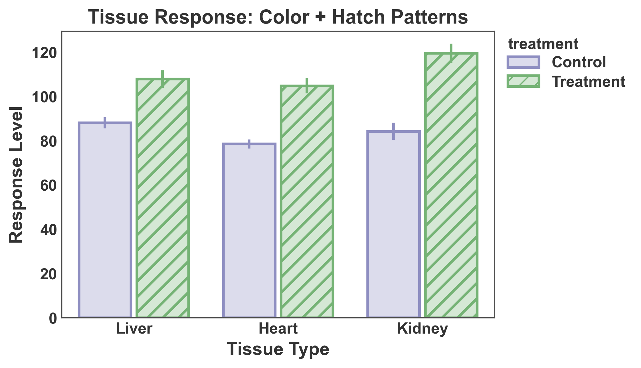
Hatch + Color for Maximum Distinction

Combine hatch patterns with colors for figures that work in both color and black-and-white formats.

# Create treatment data
np.random.seed(666)
treatment_data = pd.DataFrame({
    'tissue': np.repeat(['Liver', 'Kidney', 'Heart'], 15),
    'treatment': np.tile(['Control']*7 + ['Treatment']*8, 3),
    'response': np.concatenate([
        # Liver
        np.random.normal(85, 8, 7),    # Control
        np.random.normal(110, 12, 8),  # Treatment
        # Kidney
        np.random.normal(90, 9, 7),    # Control
        np.random.normal(115, 13, 8),  # Treatment
        # Heart
        np.random.normal(80, 7, 7),    # Control
        np.random.normal(105, 11, 8),  # Treatment
    ])
})

# Set hatch mode
pp.set_hatch_mode(3)

# Create bar plot with both color and hatch
fig, ax = pp.barplot(
    data=treatment_data,
    x='tissue',
    y='response',
    hue='treatment',
    hatch='treatment',
    title='Tissue Response: Color + Hatch Patterns',
    xlabel='Tissue Type',
    ylabel='Response Level',
    errorbar='se',
    palette={'Control': '#8E8EC1', 'Treatment': '#75B375'},
    hatch_map={'Control': '', 'Treatment': '//'},
    alpha=0.3,
)
plt.show()

# Reset mode
pp.set_hatch_mode()